


You already understand at a high level what a media mix model is and why marketers should care. Let’s get into what it takes to build a working media mix model.
This post assumes you have access to machine learning modeling resources. If you don’t, feel free to sign up for the G2M platform, our no-code modeling tool. We illustrate the media mix modeling steps below with G2M platform examples, but you can follow the same steps with any other modeling tool, such as a Jupyter notebook or another machine learning platform.
The five steps to building a media mix model
Building a media mix model involves five steps. We will cover the process end to end. If you are interested primarily in technical topics, such as algorithm selection, go straight to Step 4.
- STEP 1: Create a dataset. Compile an aggregated dataset ready to use by your model.
- STEP 2: Create a model. Create a media mix model instance in your platform of choice.
- STEP 3: Explore your dataset. Explore and validate the dataset prior to using it in your model.
- STEP 4: Configure and train your model. Select relevant variables and choose an algorithm so you can start training your media mix model.
- STEP 5: Optimize using your model. Use your media mix model to optimize your media spend.
While some analysts will complete Step 3 (data exploration) before Step 2 (model creation), we go through this specific order here, as it is more efficient to do so when working from a single tool. In practice, you may find it helpful to go through a fair amount of data exploration on your own prior to using any modeling tool.
STEP 1: Create a dataset for your media mix model
Take the time to assemble a dataset combining the outcome variable you are trying to model (e.g., whether a prospect will respond to a marketing campaign), with all the relevant attributes you know about each prospect. By way of illustration, we will use this Marketing Mix dataset, a publicly available dataset. While this dataset is ready to use for modeling, in practice you may spend a fair amount of time compiling your own dataset.
Best practices for compiling datasets will be the subject of a future post. You will need to use a combination of database platforms such as Snowflake, Amazon Redshift, Azure Synapse, or Google Big Query, and your business intelligence tool of choice such as Tableau, PowerBI, or Looker.
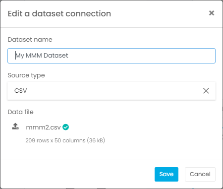
Once you’ve assembled your dataset, if you are using a Jupyter notebook, this is the part in your notebook where you would add a line of code to load your dataset. If you are using the G2M platform, you will simply go the Datasets page and create a new dataset using the CSV file that contains your data. In our example, we are using the CSV file that we downloaded of the Marketing Campaign dataset.
STEP 2: Create a media mix model
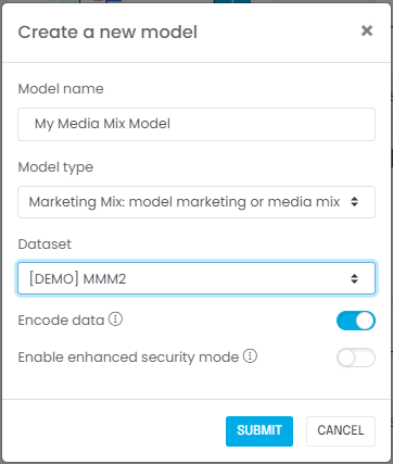
Next, you will create a model associated with your dataset. If you are using a Jupyter notebook, this is when you import the relevant machine learning libraries such as scikit-learn or Lightweight MMM. If you are using the G2M platform, you simply go to the Models page and create a new model:
STEP 3: Explore your dataset
It is important to validate that you have the right dataset, and establish some observations or hypotheses about the outcome you are trying to predict. You should also ask yourself the following questions:
- Is the sample size adequate? In most cases you will need at least a hundred rows to produce meaningful results, e.g. two years of weekly data. In our example using the media mix dataset, there are more than 200 records, so we should be fine.
- Did you include known major business drivers in the dataset? For instance pricing is almost always a meaningful driver of sales; if you made impactful pricing changes in the recent past you should include a variable capturing price changes. Other examples may include consumer confidence, unemployment, etc.
- Are you aware of meaningful changes over time that would affect the learning process? In other words, are you confident we can infer today’s behavior using yesterday’s data? In our example, the answer is “yes,” because we do not expect customer behavior to change.
- Last but not least, did you ingest the correct dataset properly? Does it look right in terms of number of rows, values appearing, etc.? It is fairly common for data to be corrupted if it is not handled using a production-grade process.
Congratulations! Now that you’ve answered these questions, you are ready to configure your media mix model.

STEP 4: Configure and train your media mix model
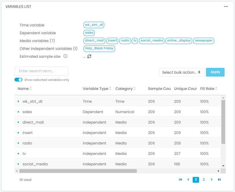
In this step, we will start by selecting variables and an algorithm. We will then train our model to interpret the results. You will need to identify and select four types of variables:
- A time variable: this variable identifies the time period of each row in the dataset. For media modeling it should be preferably weekly data. This column in the dataset should contain a date. The dataset will be sorted by ascending dates.
- A dependent variable: This is the outcome you are trying to analyze and optimize. For most media mix models, it should be a sales KPI of interest. Our dependent variable will be “sales,” the variable in the dataset that captures sales outcomes.
- Media variables: these variables will capture your media spend by media channel or type, and are handled differently than other independent variables to account for lagging and saturation effects that are common with media spend.
- Other independent variables: These are your other model inputs, and capture other variables you want to control for, such as pricing, macro-economic factors, timing of holidays, etc.
Next, you will need to consider the following data manipulation issues. If you are using a Jupyter notebook, you would select the relevant columns of a data frame.
- What is the fill rate for the variables you selected? If you combine too many variables with low fill rates (i.e., a lot of missing values), the resulting dataset will have very few complete rows unless you fill in missing variables (see below).
- If you have missing values, what in-fill strategy should you consider? The most common strategies are (i) exclude empty values, (ii) replace empty values with zeros, (iii) replace empty values with the median of the dataset if the variable is numerical, or (iv) replace empty values with the “Unknown” label if the variable is categorical. Using option (ii) or option (iii) usually requires considering what the variable actually represents. For instance, if the variable represents the number of times a customer contacted support, it would be reasonable to assume an empty value means no contact took place and replace empty values with zeros. If the variable represents the length of time a customer has been with the company, using a median might be more appropriate. You will need to use your domain knowledge for this.
- Make sure you split your data into a training set and a testing set. You will train your model on the training set and validate results using the testing set. Keep in mind that because media mix modeling datasets can be relatively small, the test period should be kept to a minimum, such as the last 13 weeks available in your data. There are several cross-validation techniques to do so efficiently; these are beyond the scope of this guide. Modeling tools such as the G2M platform will handle training and validation seamlessly and transparently.
These data manipulations are typically tedious with Jupyter notebooks but can be done straightforwardly with several tools, including the G2M platform. In our example using the media mix modeling dataset, you will end up with 1 time variable, 1 dependent variable, 7 media variables, and 1 other independent variable selected:
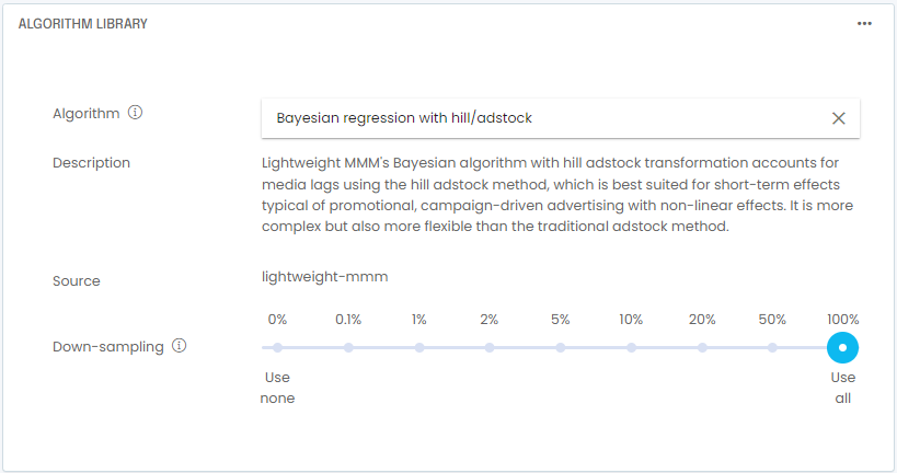
Once you’ve selected and pre-processed your variables, you will need to select an algorithm. The most common choices are:
- Naive linear regression. Using a standard linear regression is almost never the right choice as it fails to capture lagging and saturation. We recommend against using it.
- Bayesian regression with adstock effects. Bayesian modeling with adstock transformation is often the default media mix model choice. It accounts for media lags using the adstock method, which is best suited for short-term effects typical of promotional, campaign-driven advertising. Keep in mind it generally doesn’t capture saturation properly.
- Bayesian regression with Hill/adstock effects. Bayesian modeling with Hill adstock transformation accounts for media lags using the Hill adstock method, which is best suited for short-term effects typical of promotional, campaign-driven advertising with non-linear effects such as saturation. It is more complex but also more flexible than the traditional adstock method.
- Bayesian regression with carryover effects. Bayesian modeling with carryover transformation accounts for media lags using the carryover method. It is best suited to capture the longer lags seen in brand-based advertising and/or complex B2B buyer journeys.
In our example using the media mix modeling dataset, we will select the Bayesian regression with Hill/adstock algorithm:
With your variables and algorithm selected, you are now ready to train your model. In a Jupyter notebook, you typically train by invoking the fit() function. In a no-code tool such as the G2M platform, you simply go to the Train Model screen and click start. Once training is complete, you will compare actual to predicted sales over time. You will also get a set of error metrics:
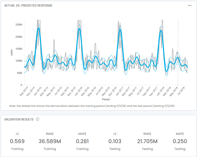
At the bottom of the example above, you also see error metrics that are typical of most media mix models:
- r2: the Pearson r2, defined as the square of the Pearson correlation, is a measure of whether there is any linear relationship between predicted and actual outcomes. It ranges from 0 to 1. In cases with strong model bias you may have low R2 and high r2: the predictions may be not good due to their bias but there is a straightforward relationship between the biased predictions and the actual outcomes.
- RMSE: the root mean square error (RMSE) measure the average difference between predicted outcomes and actual outcomes. It is defined mathematically as the standard deviation of the residuals. It is used by many regression algorithms as the objective function to be minimized.
- MAPE: the mean absolute percentage error (MAPE) is very similar to MAE and is defined as the average absolute percentage value of the difference between predictions and actuals. The value is expressed as a number, not a percentage, meaning that 100 means 1e2 and not 100%. In cases where actual outcomes are small MAPE can be quickly biased to be very large as the averaging is not weighted.
Next you will want to look at attribution and ROI to understand the relative effectiveness and different media channels:
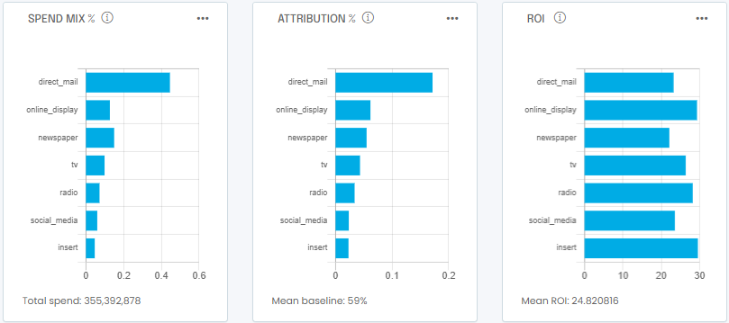
In this example you can see that the media budget is spent mostly on direct mail (left). As a result most of the sales are attributed to direct mail too (center). However, online display is a better ROI (right) and would yield more sales per incremental dollar spent.
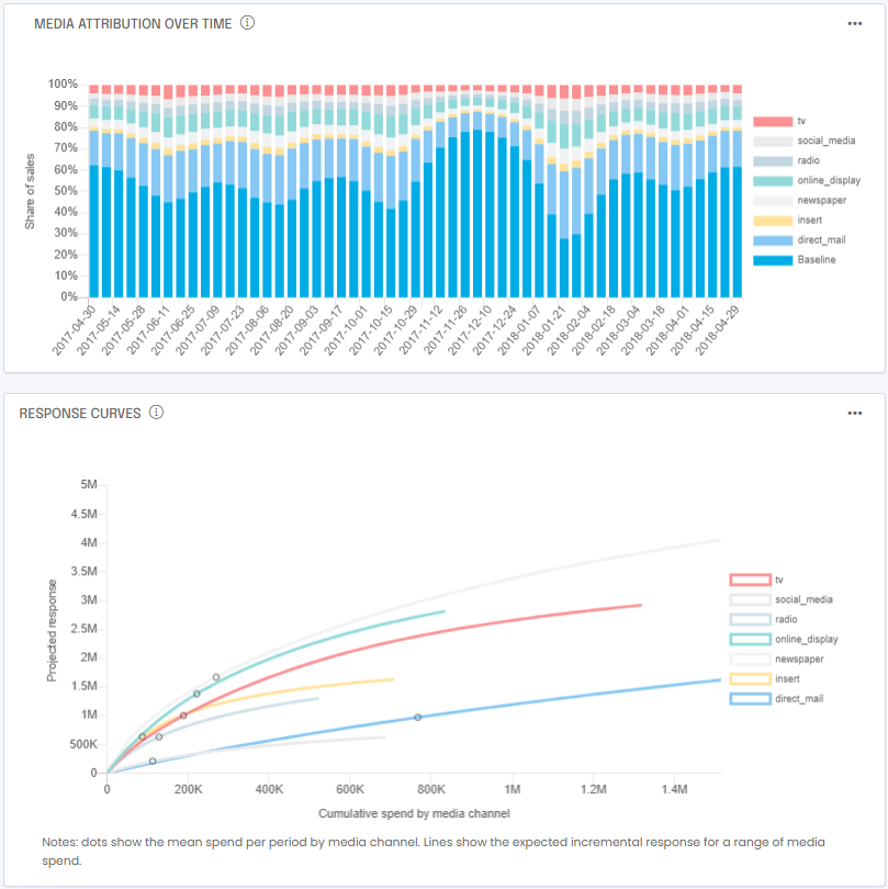
You also typically want to look at how attribution changes over time in response to changes you might have made in your media budget and response curves to understand how saturated some media channels might be:
Note that you may end up with slightly different results due to random sampling of the data when splitting your dataset into a training set and a validation set. If you’ve made it to this point, congratulations! Your model is now trained.

STEP 5: Optimize using your media mix model
You are now ready to optimize your media budget. To do so, you will typically invoke the minimize() function in a Jupyter notebook or point and click in a no-code tool such as the G2M platform. As you use your model over time, keep in mind the issue of model drift. See this post for an explanation of model drift. We will cover optimization in detail in a future post.
How Can We Help?
Feel free to check us out and start your free trial at https://app.g2m.ai or contact us below!
